What is trace, really?

The trace of a square matrix is defined as the sum of its diagonal entries. This definition can look a little mysterious at first. Why do we single out only the diagonal entries of a matrix, and why do we add them?

The short answer is that trace is, in essence, "a product with itself." In other words, trace is the operation of connecting the output and input of a linear map to make a "loop." Below, we explain what these slogans mean.

Definition of trace

Let us first recall the usual definition. For an \(n\)-by-\(n\) square matrix \(A=(a_{ij})_{1\le i,j\le n}\) over a field \(k\), the trace of \(A\) is defined by

\[ \operatorname{tr}(A)=\sum_{i=1}^n a_{ii} \]

In other words, it is the sum of the diagonal entries running from the upper left to the lower right. For example, if

\[ A=\begin{pmatrix} 2&1&0\\ 3&-1&4\\ 5&2&7 \end{pmatrix}, \]

then \(\operatorname{tr}(A)=2+(-1)+7=8\).

If we look only at the definition, the operation "add the diagonal entries" may feel unnatural. A matrix has many other entries, so why do we pick out only \(a_{11},a_{22},\ldots,a_{nn}\)? The key to answering this question lies in the concept of matrix multiplication.

Matrix multiplication

The product of an \(m\times n\) matrix \(A=(a_{ij})_{1\le i\le m,1\leq j\le n}\) and an \(n\)-dimensional column vector \(x=(x_i)_{1\leq i\le n}\) is given by

\[ (Ax)_i=\sum_{j=1}^n a_{ij} x_j \]

Let us draw this formula as follows.

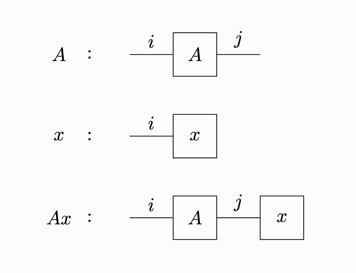
Diagram of the product of a matrix and a vector

In words, the diagram means the following.

The matrix \(A\) is drawn as a box with one string extending from each side. The left string represents the row index, and the right string represents the column index.
The vector \(x\) is drawn as a box with one string extending to the left. The left string represents the row index.
Connecting strings means summing over the corresponding index.

This last operation, summing over a connected index, is called contraction.

Matrix multiplication can be drawn in the same way. For an \(m\times n\) matrix \(A=(a_{ij})_{1\le i\leq m,1\leq j \leq n}\) and an \(n\times\ell\) matrix \(B=(b_{ij})\), their product \(AB\) is given by

\[ (AB)_{ik}=\sum_{j=1}^n a_{ij}b_{jk} \]

Thus the formula can be represented by the following diagram.

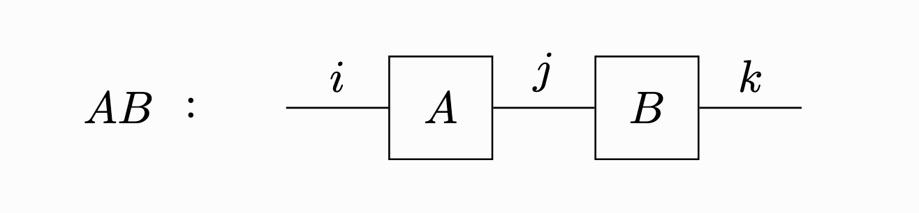
Similarly, products such as the product \(ABC\) of three matrices, or the product \(ABx\) of two matrices and a vector, can also be represented diagrammatically from their component formulas.

Trace is a loop

Now consider an \(n\)-by-\(n\) square matrix \(A=(a_{ij})_{1\le i,j\le n}\). As described above, this corresponds to a diagram with two strings coming out of one box. Let us connect these two strings to make a loop.

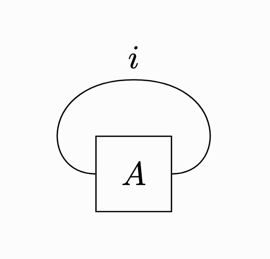
Then the corresponding formula is obtained by summing over the connected index \(i\), so it is

\[ \sum_{i=1}^n a_{ii} \]

This is exactly the definition of the trace of \(A\). Thus trace is the result of contracting the input-side index and the output-side index of the matrix \(A\), just as in matrix multiplication. This is the meaning of the slogan stated at the beginning: "trace is a product with itself."

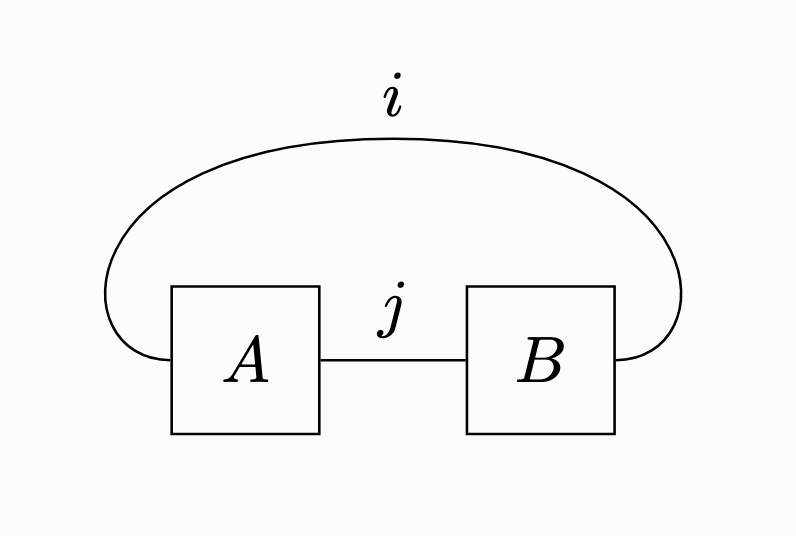
When we regard trace as a loop in this way, the identity

\[ \operatorname{tr}(AB)=\operatorname{tr}(BA) \]

for an \(m\times n\) matrix \(A\) and an \(n\times m\) matrix \(B\) also becomes natural. Written as a diagram, this corresponds to the fact that \(B\) can move along the upper side of the loop to the left side of \(A\).

More generally, suppose that matrices \(A_1,\dots,A_N\) are such that the products \(A_iA_{i+1}\) are defined for \(i=1,2,\dots,N\), where we set \(A_{N+1}=A_1\). Then the same explanation gives the invariance under cyclic permutation

\[ \operatorname{tr}(A_1A_2\cdots A_{N-1}A_N)=\operatorname{tr}(A_NA_1A_2\cdots A_{N-1}). \]

From this property, it is also immediate that trace is invariant under similarity of matrices. Indeed, for an \(n\)-by-\(n\) square matrix \(A\) and an invertible matrix \(P\),

\[ \operatorname{tr}(P^{-1}AP) =\operatorname{tr}(PP^{-1}A) =\operatorname{tr}(A). \]

If we draw the diagram, we see that this corresponds to the simple principle that \(P\) and \(P^{-1}\) sit next to each other on the loop and cancel.

Basis-free definition

So far we have used component expressions for matrices, but in fact trace can be defined without using components, purely in the language of abstract linear maps. For a finite-dimensional vector space \(V\), let \(V^*\) be its dual space. Then there is a canonical isomorphism

\[ V^*\otimes V \cong \operatorname{End}(V). \]

Concretely, it sends a simple tensor \(\varphi\otimes v\in V^*\otimes V\) to the linear map

\[ x\mapsto \varphi(x)v. \]

Extending this correspondence linearly gives an isomorphism between \(V^*\otimes V\) and \(\operatorname{End}(V)\). Using this, define the linear map \(\operatorname{coev}\colon k\to V^*\otimes V\), called coevaluation, as follows:

\[ \operatorname{coev}\colon k\xrightarrow{1\mapsto \mathrm{id}_V} \operatorname{End}(V)\cong V^*\otimes V. \]

Also define the linear map \(\operatorname{ev}\colon V^*\otimes V\to k\), called evaluation, as follows:

\[ \operatorname{ev}\colon V^*\otimes V\to k;\quad \varphi\otimes v\mapsto \varphi(v). \]

Then, for a linear map \(f\colon V\to V\), the following composite agrees with multiplication by \(\operatorname{tr}(f)\):

\[ k \xrightarrow{\operatorname{coev}} V^*\otimes V \xrightarrow{\mathrm{id}\otimes f} V^*\otimes V \xrightarrow{\operatorname{ev}} k. \]

Let us verify the claim above. Take a basis \(e_1,\ldots,e_n\) of \(V\) and its dual basis \(e_1^*,\ldots,e_n^*\), and let \(A=(a_{ij})_{1\le i,j\le n}\) be the matrix of the linear map \(f\colon V\to V\) with respect to this basis. Then the element of \(V^*\otimes V\) corresponding to the identity map \(\mathrm{id}_V\colon V\to V\) is

\[ \sum_{i=1}^n e_i^*\otimes e_i. \]

Therefore coevaluation sends \(1\) to this element. Applying \(\mathrm{id}\otimes f\) further gives

\[ \sum_{i=1}^n e_i^*\otimes f(e_i) = \sum_{i=1}^n\sum_{j=1}^n e_i^*\otimes a_{ji}e_j. \]

Applying evaluation, and using \(e_i^*(e_j)=\delta_{ij}\), we obtain

\[ \sum_{i=1}^n a_{ii} = \operatorname{tr}(A). \]

Thus the composite map \(k\to k\) above is equal to multiplication by \(\operatorname{tr}(f)\).

Trace in string diagrams

The interpretation of trace as a "loop" from two sections ago and the definition of trace using evaluation and coevaluation from the previous section may look completely different at first. In fact, however, if we draw the latter definition using a method called a "string diagram," the loop appears exactly as before.

A string diagram is a way of depicting objects and morphisms in a category equipped with a "tensor product" (a monoidal structure), such as the category of vector spaces. We will not go deeply into the precise rules for drawing string diagrams here. It is enough to keep only the following rules in mind.

A vector space is represented by a vertical line.
The tensor product of vector spaces is represented by placing vertical lines side by side.
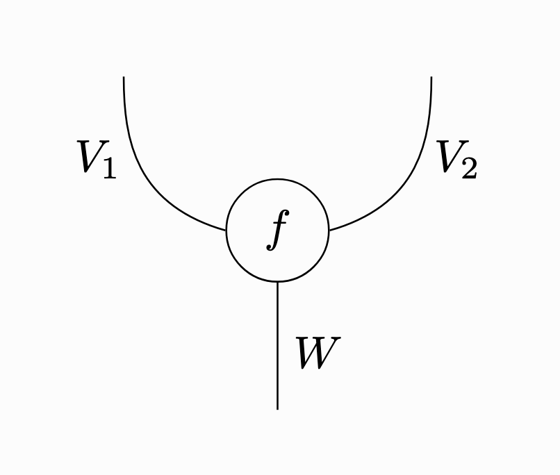
A linear map is represented by a junction connecting vertical lines from top to bottom.
The vertical line representing the vector space \(k\) is omitted.

For example, for vector spaces \(V_1,V_2,W\), a linear map \(f\colon V_1\otimes V_2\to W\) is represented by the following string diagram.

With this in mind, the abstract definition of trace from the previous section,

\[ k \xrightarrow{\operatorname{coev}} V^*\otimes V \xrightarrow{\mathrm{id}\otimes f} V^*\otimes V \xrightarrow{\operatorname{ev}} k \]

is drawn as the following string diagram.

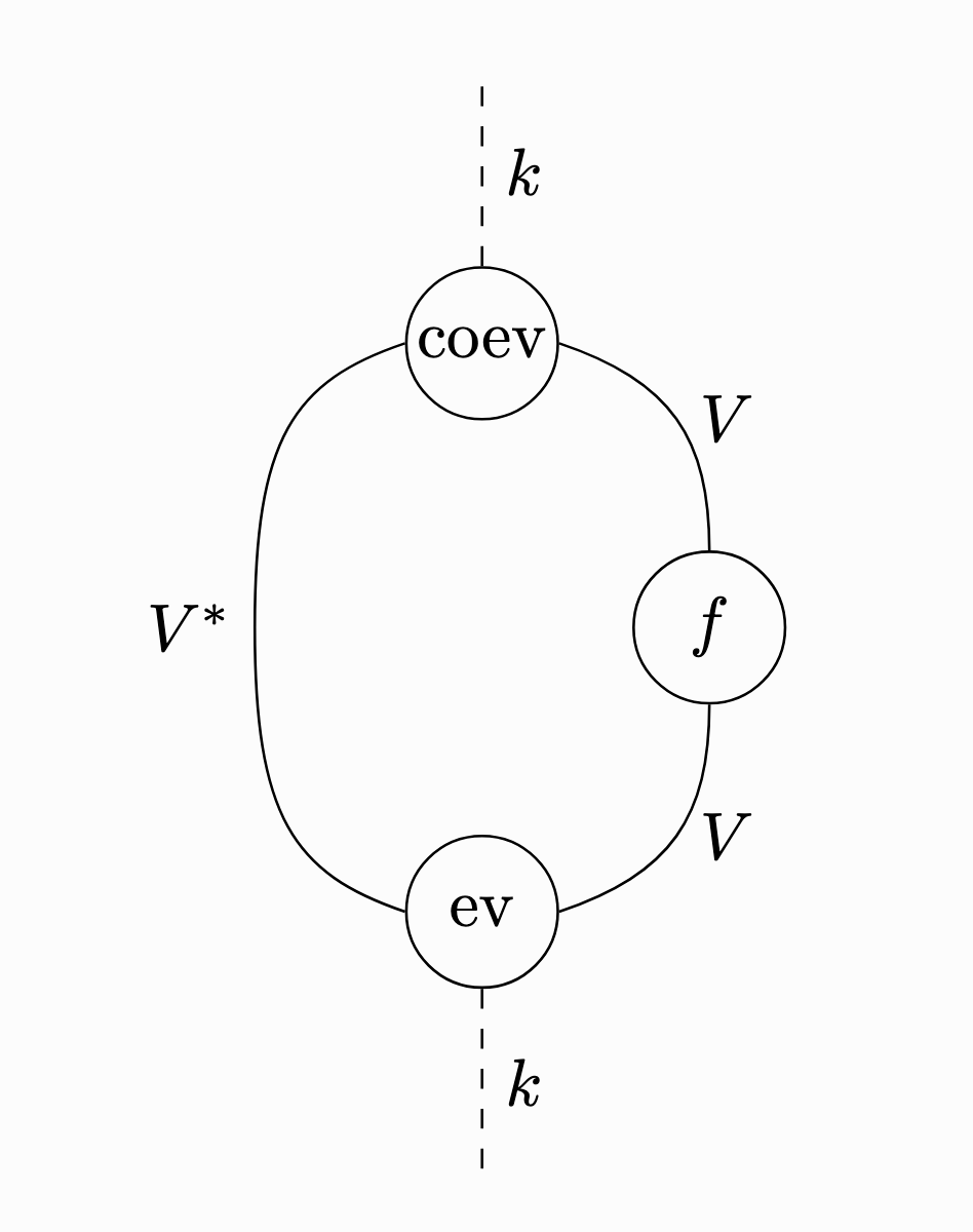
String diagram of trace using evaluation and coevaluation

We can see the two strings coming out of \(f\) being bent by evaluation and coevaluation to form a loop. In other words, the definition of trace given in the previous section is precisely the categorical version, expressed through string diagrams, of the intuition of a "loop."

Fixed points and trace

One important place where trace appears in mathematics is the Lefschetz trace formula. Let \(M\) be an oriented compact manifold, and consider a smooth map \(f\colon M\to M\). A point \(x\in M\) satisfying \(f(x)=x\) is called a fixed point of \(f\). As a technical assumption, suppose that the fixed points of \(f\) do not accumulate. Then the Lefschetz trace formula says that the sum, over the fixed points of \(f\), of certain signed quantities called local fixed point indices is given by

\[ \sum_{i=0}^\infty (-1)^i \operatorname{tr}(f^*|H^i(M;\mathbb{Q})). \]

Here \(f^*\) is the map induced by \(f\) on cohomology groups:

\[ f^*\colon H^i(M;\mathbb{Q})\to H^i(M;\mathbb{Q}). \]

Roughly speaking, the Lefschetz trace formula is a formula that connects fixed points and traces.

The fact that trace is related to fixed points also becomes natural from the picture of "contracting input and output" described in the preceding sections. As a simple example, let us consider a self-map of a finite set.

\[ X=\{1,2,\ldots,n\} \]

Let \(f\colon X\to X\) be a self-map. Identifying an element \(i\in X\) with the standard basis vector \(e_i\) of \(k^n\), \(f\) induces a linear map \(k^n\to k^n\). Let \(A_f\) be the matrix of this linear map. Concretely, if \(A_f=(a_{ij})_{1\le i,j\le n}\), then

\[ a_{ij}= \begin{cases} 1&(i=f(j))\\ 0&(i\neq f(j)) \end{cases} \]

Taking the trace of this matrix gives

\[ \operatorname{tr}(A_f) =\sum_{i=1}^n a_{ii} =\#\{i\in X\mid f(i)=i\}. \]

Thus the number of fixed points of \(f\) appears. In this computation, "contracting input and output" in the definition of trace corresponds exactly to requiring "input and output to agree" in the definition of a fixed point. Therefore, in a certain sense, we may also say that trace is a generalization of the number of fixed points.

Acknowledgments

The slogan emphasized in this article, "trace is a product with itself," is borrowed from Kyosuke Higashida. I thank him for sharing such a good phrase.